Discuss
Specialists translate market needs into geometry and simulation questions.
Collapse a slow, expert-heavy engineering loop into rapid design exploration and tolerance-linked manufacturing decisions.
Today, computational physicists, mechanical engineers and market leaders must align before a design can move. For an FT Technologies wind sensor, that decision sits across aerodynamic, thermal and acoustic behaviour—nonlinear simulations that can take days before the team gets the evidence needed for its next discussion.
Specialists translate market needs into geometry and simulation questions.
Coupled simulations take time, delaying the evidence needed for a decision.
Every new manufactured design adds cost before the next learning cycle begins.
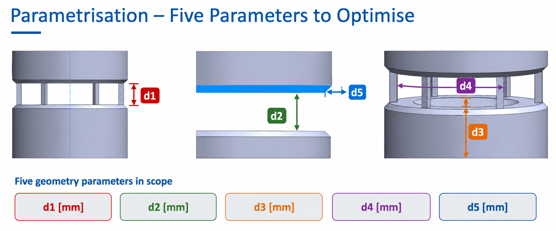
Five geometry parameters connect design intent, predicted response and manufacturing inspection.
Forward LightGBM surrogate — geometry → acoustic response Instead of waiting for another full physics run, the surrogate gives the team an immediate view of how a proposed geometry shifts resonance position, amplitude and width.
After extensive feature studies and evaluation, the response was represented as a baseline plus up to three fitted Gaussian resonances. The model predicts those physically meaningful shape parameters—not 360 unrelated pressure values—and reconstructs the complete curve.
Stay inside the learned design space.
Controls are limited to the geometry ranges used to train the model.
Inverse 1D CNN inspector — measured response → inferred geometry The convolutional model reads the complete 61-point sweep, learning resonance shapes and spacing across frequency to infer the five dimensions that most likely produced it.
This closes the loop between modelling and manufacturing. A measured part can be compared with its known reference geometry and actual engineering tolerance, producing an immediate dimension-by-dimension pass/fail view.
Choose a held-out test example to compare the CNN estimate with its known geometry.